Parameter, Statistic, Random Variable, Estimator and Estimate
The most common problem while learning Statistics is that students’ lack of understanding of the basic terminologies, notations, definitions and concepts. Think of Statistics as building blocks, and you need a solid foundation to move forward. Here, I explain five common terms in Statistics: i) Parameter, ii) Statistic, iii) Random Variable, iv) Estimator, v) Estimate and their notations.
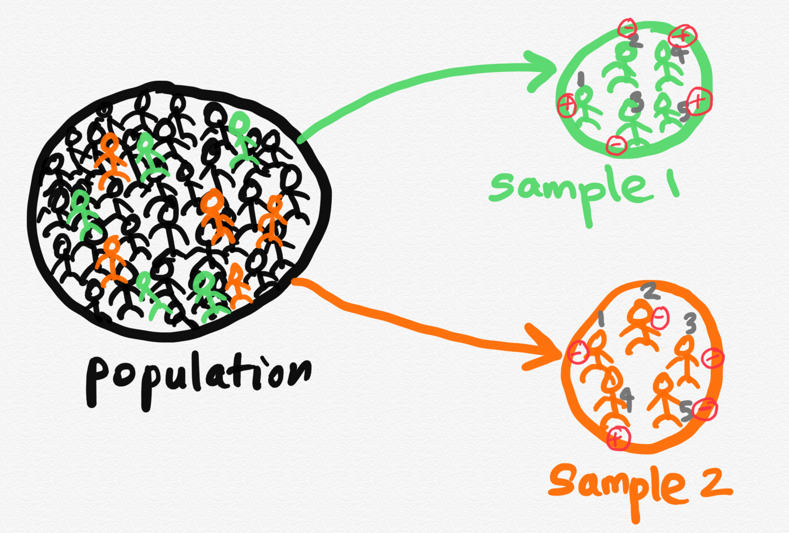
I will start with the definition of Population and Sample.
A population is a complete collection of individuals/ objects that we are interested in. A sample is a subset of a population.
Parameter
A parameter is a descriptive measure(numerical value) of the population. Parameters are usually denoted by Greek letters.
Examples of parameters:
\(\mu\) - population mean
\(\sigma^2\) - population variance
Statistic
A statistic is a descriptive measure of a sample. For example, sample mean, sample standard deviation, etc. We will talk about the notations under estimator and estimate.
Random Variable
Before introducing random variable, let me very shortly recall what is a random experiment and what is a sample space.
A random experiment is a physical situation whose outcome cannot be predicted with certainty until it is observed. A random experiment can be repeated as many times as we want under the same conditions (leading to different outcomes). Each one of them a trial. Thus, a trial is a particular performance of a random experiment.
A Sample space is a set of all possible outcomes of a random experiment. In this blog post I use \(\Omega\) to denote a sample space.
Example 1:
Random Experiment: Tossing of a coin.
Sample Space: \(\Omega = \{H, T\}\)
library(prob)
tosscoin(1)
toss1
1 H
2 TExample 2:
Random Experiment: Toss a coin three times.
Sample Space: \(\Omega = \{(H, H, H), (H, H, T), (H, T, H), (T, H, H), (H, T, T), (T, H, T), (T, T, H), (T, T, T)\}\)
tosscoin(3) toss1 toss2 toss3
1 H H H
2 T H H
3 H T H
4 T T H
5 H H T
6 T H T
7 H T T
8 T T TDefinition: Random Variable
Let \((\Omega, \mathscr{F}, \mathbb{P})\) be a probability space. Random variable is a function \(X: \Omega \rightarrow \mathbb{R}\) such that \(\forall B \in \mathcal{B}( \mathbb{R} ): X^{-1}(B) \in \mathscr{F}\).
You need Measure Theory knowledge to understand the above definition.
Loosely speaking a Random variable is a function from the sample space to the real numbers. There are two types of random variables: i) Discrete random variable and ii) Continuous random variable. We use Roman capital letters to denote random variables (\(X\), \(Y\), \(Z\), \(U\), \(T\), etc.). However, as soon as a variable \(X\) is observed, the observed values are represented by the corresponding simple Roman letter.
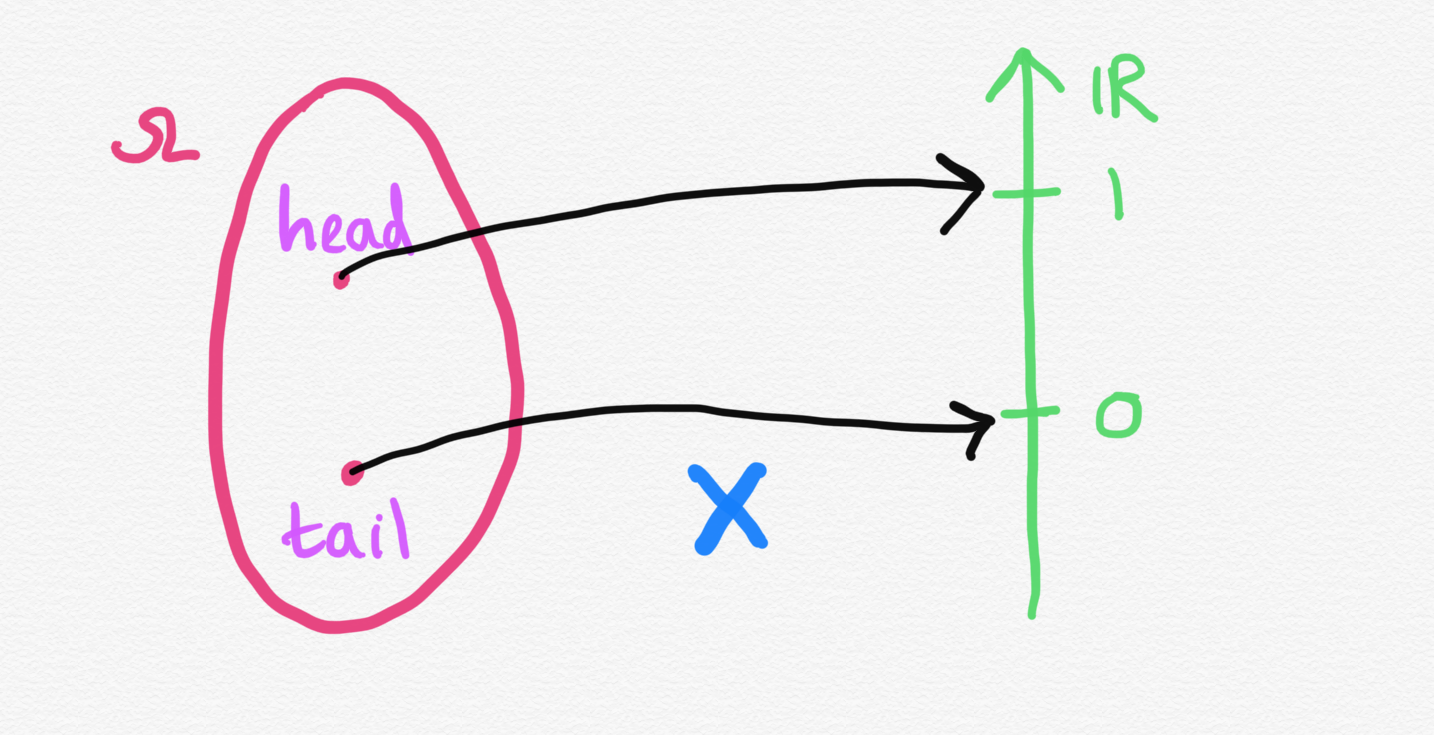
The notation \(X(\omega)\) denotes the numerical value of the random variable X, when the outcome of the experiment is some particular \(\omega\).
An example will help you to understand how this works. To start with, let’s consider a simple experiment with two possible outcomes: PCR test result of a randomly selected individual.

The random variable \(X\) can be defined as follows:
Solution 1.1
Sample space
\[\Omega = \{Positive, Negative\}\]
Random variable
\[ X(\omega)= \begin{cases} 0,& \text{if } \omega = Negative\\ 1, & \text{if } \omega = Positive \end{cases} \]
Solution 1.2
Simply drop \(\omega\) and define the random variable as follows:
\[ X= \begin{cases} 0,& \text{if the test result is negative. } \\ 1, & \text{if the test result is positive.} \end{cases} \]
Let’s consider another experiment. The experiment consists in selecting a random undergraduate student in the University during a period of one week, and measuring their height.
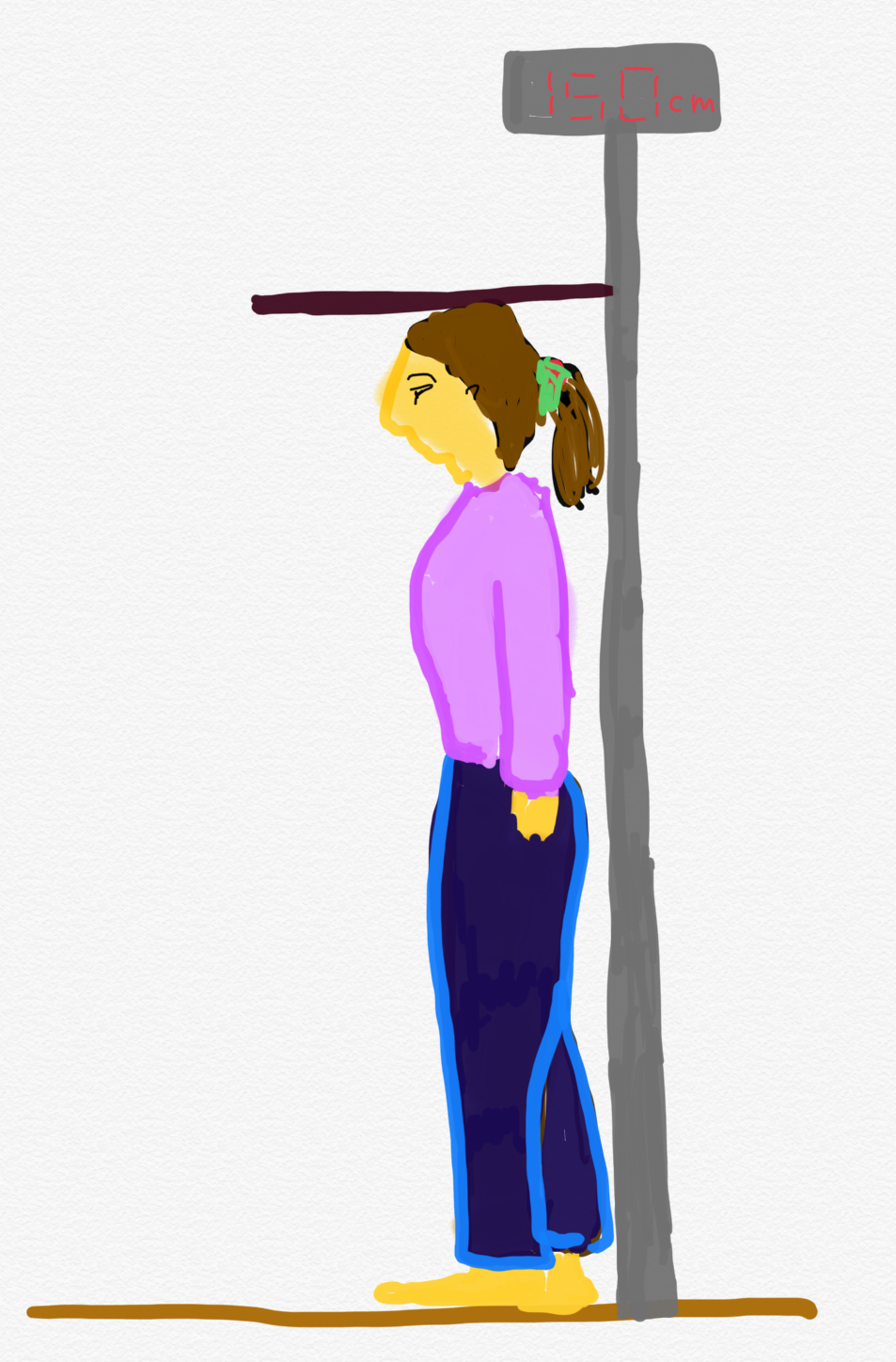
The random variable \(Y\) can be defined as follows:
\[\Omega = \{ \omega: \omega > 0\}\]
\[Y(\omega) = \omega, \text{ } \omega \in \Omega. \]
or
\[Y = \text{Height in cm.}\]
Notations for Random Variables and Observed Data (in Sampling)
Suppose you have a random variable \(X\). Suppose we repeat the random experiment \(n\) times. Then the resulting random variables are denoted by \(X_1, X_2, ..., X_n\). All \(X_i\)’s have the same distribution as \(X\). The random variables \(X_1, X_2, ..., X_n\) are collectively referred to as a random sample.
Let’s try to understand the concept with an example.
\[ X_i= \begin{cases} 0,& \text{if the test result of the } i^{th} \text { is negaive } \\ 1, & \text{if the test result of the } i^{th} \text { is positive, } \end{cases} \]
where \(i = 1, 2, 3, 4, 5.\)
We performed the PCR test on randomly selected 5 individuals. We called this sample 1. The results are \(x_1=1, x_2=0, x_3=0, x_4=1, x_5=1\).
Prior to obtaining \(x_1, x_2, x_3, x_4, x_5\), there is uncertainty about the values of each \(x_i\). Because of this uncertainty, before the results becomes available we view each observation as a random variable and denote the sample by \(X_1, X_2, X_3, X_4, X_5\).
We again performed the PCR test on another randomly selected 5 individuals. We called this sample 2. Now results are \(x_1=0, x_2=0, x_3=0, x_4=1, x_5=0\).
You can see observable values for \(X_1, X_2, X_3, X_4, X_5\) vary from sample to sample.
Estimator and Estimate
Distinction between the terms Estimator and Estimate is important.
Let \(X_1, X_2, ..., X_n\) be a random sample from a distribution function \(f_X(x)\) that depends on a unknown parameter \(\theta\).
An estimator is a statistic, \(T = f(X_1, ..., X_n)\), that is used to estimate the unknown unknown parameter, \(\theta\), based on an observed sample of \(x_1, x_2, ..., x_n\). The \(t=f(x_1, x_2, ..., x_n)\) is an estimate of \(\theta\).
Estimator: An estimator is always a random variable.
\(\hat{\theta} = T = f(X_1, ..., X_n)\)
Estimate: An estimate is a constant.
\(\hat{\theta} = t = f(x_1, ..., x_n)\)
Note that we use \(\hat{\theta}\) for both estimator and estimate.
Estimator is a function of observable random variables that is used to estimate an unknown parameter \(\theta\). The corresponding estimate is obtained by substituting the observed values to the estimator. You can also think of an estimator as the rule (equation) that is used to compute an estimate. For example, the sample mean, \(\bar{X}\), is an estimator that is used to estimate the population mean, \(\mu\).
Below example is useful to understand the concepts.
Let’s say you wanted to know the mean height of undergraduates in a certain university with a population of 1000 undergraduates. You take a random sample of 10 students and measure their height. The observed values are (in cm) 150, 155, 160, 161, 162, 152, 140, 141, 150, 155. Suppose you want to use sample mean to estimate the population mean.
The parameter we want to estimate is, \(\mu\), population mean (mean height of the students in the university.).
There are infinitely many possible estimators for \(\mu\). For example, sample mean, sample median. In this example we use sample mean to estimate \(\mu\). Now, let’s write the estimator using the notations.
To do this, we first define random variables \(X_1, X_2, X_3, ..., X_{10}\) as follows: \(X_1\) is the height of the \(1^{st}\) chosen person, \(X_2\) be the height of the \(2^{nd}\) chosen person,…. In general, \(X_i\) is the height of the \(i^{th}\) student chosen from the population.
Now we can write the estimator as
\[\hat{\mu} = \bar{X}=\frac{X_1 + X_2 + X_3 + ... + X_{10}}{10}.\]
The estimate is
\[\hat{\mu}=152.6\text{ cm}.\]
mean(c(150, 155, 160, 161, 162, 152, 140, 141, 150, 155))[1] 152.6If you are not given the observed values of \(X_1, X_2, X_3, ..., X_{10}\), you can write the estimate as
\[\hat{\mu} = \frac{x_1 + x_2 + x_3 + ... + x_{10}}{10}.\]
The observed value of the estimator varies from sample to sample.
Usage
- Writing distributions
\[X \sim Bin(10, 0.6)\]
\[f_X(x) = P(X=x) = {10\choose x} 0.6^x 0.4^{(10-x)}\]
\[f_X(5) = P(X=5) = {10\choose 5} 0.6^5 0.4^{(10-5)} = 0.37\]
pbinom(5, 10, 0.6)[1] 0.3668967- Calculation of expectations
\[E(\text{Estimator}) = \text{Parameter}\]
\[E(\bar{X}) = \mu\]
 This work is
licensed under a Creative Commons Attribution 4.0 International
License.
This work is
licensed under a Creative Commons Attribution 4.0 International
License.