STA 517 3.0 Programming and Statistical Computing with RRegression AnalysisDr Thiyanga Talagala25 October 20201 / 82

2 / 82

Packages

library(broom)
library(modelr)
library(GGally)
library(carData)
library(tidyverse)
library(magrittr)
library(car) # to calculate VIF

3 / 82

Data: Prestige of Canadian Occupations

head(Prestige, 5)

                    education income women prestige census type
gov.administrators      13.11  12351 11.16     68.8   1113 prof
general.managers        12.26  25879  4.02     69.1   1130 prof
accountants             12.77   9271 15.70     63.4   1171 prof
purchasing.officers     11.42   8865  9.11     56.8   1175 prof
chemists                14.62   8403 11.68     73.5   2111 prof

summary(Prestige)

   education          income          women           prestige    
 Min.   : 6.380   Min.   :  611   Min.   : 0.000   Min.   :14.80  
 1st Qu.: 8.445   1st Qu.: 4106   1st Qu.: 3.592   1st Qu.:35.23  
 Median :10.540   Median : 5930   Median :13.600   Median :43.60  
 Mean   :10.738   Mean   : 6798   Mean   :28.979   Mean   :46.83  
 3rd Qu.:12.648   3rd Qu.: 8187   3rd Qu.:52.203   3rd Qu.:59.27  
 Max.   :15.970   Max.   :25879   Max.   :97.510   Max.   :87.20  
     census       type   
 Min.   :1113   bc  :44  
 1st Qu.:3120   prof:31  
 Median :5135   wc  :23  
 Mean   :5402   NA's: 4  
 3rd Qu.:8312            
 Max.   :9517

4 / 82

Data description

prestige: prestige of Canadian occupations, measured by the Pineo-Porter prestige score for occupation taken from a social survey conducted in the mid-1960s.

education: Average education of occupational incumbents, years, in 1971.

income: Average income of incumbents, dollars, in 1971.

women: Percentage of incumbents who are women.

census: Canadian Census occupational code.

type: Type of occupation.

- prof: professional and technical
- wc: white collar
- bc: blue collar
- NA: missing

The dataset consists of 102 observations, each corresponding to a particular occupation.

5 / 82

Training test and Test set

smp_size <- 80
## set the seed to make your partition reproducible
set.seed(123)
train_ind <- sample(seq_len(nrow(Prestige)), size = smp_size)
train <- Prestige[train_ind, ]
dim(train)

[1] 80  6

test <- Prestige[-train_ind, ]
dim(test)

[1] 22  6

6 / 82

Exploratory Data Analysis

Prestige_1 <- train %>%
  pivot_longer(c(1, 2, 3, 4), names_to="variable", values_to="value")
Prestige_1

# A tibble: 320 x 4
   census type  variable    value
    <int> <fct> <chr>       <dbl>
 1   3156 wc    education   12.8 
 2   3156 wc    income    5180   
 3   3156 wc    women       76.0 
 4   3156 wc    prestige    67.5 
 5   8335 bc    education    7.92
 6   8335 bc    income    6477   
 7   8335 bc    women        5.17
 8   8335 bc    prestige    41.8 
 9   5133 wc    education   11.1 
10   5133 wc    income    8780   
# … with 310 more rows

7 / 82

Exploratory Data Analysis

Prestige_1 <- train %>%
  pivot_longer(c(1, 2, 3, 4), names_to="variable", values_to="value")
Prestige_1

# A tibble: 320 x 4
   census type  variable    value
    <int> <fct> <chr>       <dbl>
 1   3156 wc    education   12.8 
 2   3156 wc    income    5180   
 3   3156 wc    women       76.0 
 4   3156 wc    prestige    67.5 
 5   8335 bc    education    7.92
 6   8335 bc    income    6477   
 7   8335 bc    women        5.17
 8   8335 bc    prestige    41.8 
 9   5133 wc    education   11.1 
10   5133 wc    income    8780   
# … with 310 more rows

head(train)

                      education income women prestige census type
medical.technicians       12.79   5180 76.04     67.5   3156   wc
welders                    7.92   6477  5.17     41.8   8335   bc
commercial.travellers     11.13   8780  3.16     40.2   5133   wc
economists                14.44   8049 57.31     62.2   2311 prof
farmers                    6.84   3643  3.60     44.1   7112 <NA>
receptionsts              11.04   2901 92.86     38.7   4171   wc

7 / 82

Exploratory Data Analysis

ggplot(Prestige_1, aes(x=value)) + geom_histogram() + 
  facet_wrap(variable ~., ncol=1)

8 / 82

Exploratory Data Analysis

ggplot(Prestige_1, aes(x=value)) + geom_histogram() + 
  facet_wrap(variable ~., ncol=1, scales = "free")

9 / 82

Exploratory Data Analysis

ggplot(Prestige_1, aes(x=value)) + geom_histogram(colour="white") + 
  facet_wrap(variable ~., ncol=1, scales = "free")

10 / 82

Exploratory Data Analysis

ggplot(Prestige_1, aes(x=value, fill=variable)) + geom_density() + 
  facet_wrap(variable ~., ncol=1, scales = "free")

11 / 82

Exploratory Data Analysis

ggplot(Prestige_1, aes(y = value, x = type, fill = type)) + geom_boxplot() + 
  facet_wrap(variable ~., ncol=1, scales = "free")

12 / 82

Exploratory Data Analysis

Prestige_1 %>%
   filter(is.na(type) == FALSE) %>%
ggplot(aes(y=value, x=type, fill=type)) + geom_boxplot() + 
  facet_wrap(variable ~., ncol=1, scales = "free")

13 / 82

Exploratory Data Analysis

Prestige_1 %>%
  filter(is.na(type) == FALSE) %>%
ggplot(aes(x = value, y = type, fill = type)) + geom_boxplot() + 
  facet_wrap(variable ~., ncol=1, scales = "free")

14 / 82

Exploratory Data Analysis

train %>%
  select(education, income, prestige, women) %>%
  ggpairs()

15 / 82

Exploratory Data Analysis

train %>%
  filter(is.na(type) == FALSE) %>%
  ggpairs(columns= c("education", "income", "prestige", "women"),
          mapping=aes(color=type))

16 / 82

Regression analysis17 / 82

Steps

Fit a model.
Visualize the fitted model.
Measuring the strength of the fit.
Residual analysis.
Interpret the coefficients.
Make predictions using the fitted model.

18 / 82

Model 1: prestige ~ education19 / 82

Recap

True relationship between X and Y in the population

$Y = f (X) + ϵ$

If $f$ is approximated by a linear function

$Y = β_{0} + β_{1} X + ϵ$

The error terms are normally distributed with mean $0$ and variance $σ^{2}$ . Then the mean response, $Y$ , at any value of the $X$ is

$E (Y | X = x_{i}) = E (β_{0} + β_{1} x_{i} + ϵ) = β_{0} + β_{1} x_{i}$

For a single unit $(y_{i}, x_{i})$

$y_{i} = β_{0} + β_{1} x_{i} + ϵ_{i} where ϵ_{i} \sim N (0, σ^{2})$

We use sample values $(y_{i}, x_{i})$ where $i = 1, 2, . . . n$ to estimate $β_{0}$ and $β_{1}$ .

The fitted regression model is

$\hat{Y_{i}} = {\hat{β}}_{0} + {\hat{β}}_{1} x_{i}$

20 / 82

How to estimate $β_{0}$ and $β_{1}$ ?

Sum of squares of Residuals

$S S R = e_{1}^{2} + e_{2}^{2} + . . . + e_{n}^{2}$

The least-squares regression approach chooses coefficients ${\hat{β}}_{0}$ and ${\hat{β}}_{1}$ to minimize $S S R$ .

21 / 82

22 / 82

23 / 82

24 / 82

25 / 82

26 / 82

27 / 82

28 / 82

29 / 82

Model 1: prestige ~ education1. Fit a model30 / 82

Model 1: Fit a model

$y_{i} = β_{0} + β_{1} x_{i} + ϵ_{i}, where ϵ_{i} \sim N I D (0, σ^{2})$

To estimate $β_{0}$ and $β_{1}$

model1 <- lm(prestige ~ education, data=train)
summary(model1)


Call:
lm(formula = prestige ~ education, data = train)
Residuals:
     Min       1Q   Median       3Q      Max 
-26.4715  -5.8396   0.9778   6.2464  17.4767 
Coefficients:
            Estimate Std. Error t value Pr(>|t|)    
(Intercept)   -9.418      3.918  -2.404   0.0186 *  
education      5.269      0.353  14.928   <2e-16 ***
---
Signif. codes:  0 '***' 0.001 '**' 0.01 '*' 0.05 '.' 0.1 ' ' 1
Residual standard error: 8.754 on 78 degrees of freedom
Multiple R-squared:  0.7407,    Adjusted R-squared:  0.7374 
F-statistic: 222.8 on 1 and 78 DF,  p-value: < 2.2e-16

31 / 82

What's messy about the output?


Call:
lm(formula = prestige ~ education, data = train)
Residuals:
     Min       1Q   Median       3Q      Max 
-26.4715  -5.8396   0.9778   6.2464  17.4767 
Coefficients:
            Estimate Std. Error t value Pr(>|t|)    
(Intercept)   -9.418      3.918  -2.404   0.0186 *  
education      5.269      0.353  14.928   <2e-16 ***
---
Signif. codes:  0 '***' 0.001 '**' 0.01 '*' 0.05 '.' 0.1 ' ' 1
Residual standard error: 8.754 on 78 degrees of freedom
Multiple R-squared:  0.7407,    Adjusted R-squared:  0.7374 
F-statistic: 222.8 on 1 and 78 DF,  p-value: < 2.2e-16

Extract coefficients takes multiple steps.
```
data.frame(coef(summary(model1)))
```
Column names are inconvenient to use.
Information are stored in row names.

32 / 82

`broom` functions

broom takes model objects and turns them into tidy data frames that can be used with other tidy tools.
Three main functions

tidy(): component-level statistics

augment(): observation-level statistics

glance(): model-level statistics

33 / 82

Component-level statistics: `tidy()`

model1 %>% tidy()

# A tibble: 2 x 5
  term        estimate std.error statistic  p.value
  <chr>          <dbl>     <dbl>     <dbl>    <dbl>
1 (Intercept)    -9.42     3.92      -2.40 1.86e- 2
2 education       5.27     0.353     14.9  1.43e-24

model1 %>% tidy(conf.int=TRUE)

# A tibble: 2 x 7
  term        estimate std.error statistic  p.value conf.low conf.high
  <chr>          <dbl>     <dbl>     <dbl>    <dbl>    <dbl>     <dbl>
1 (Intercept)    -9.42     3.92      -2.40 1.86e- 2   -17.2      -1.62
2 education       5.27     0.353     14.9  1.43e-24     4.57      5.97

model1 %>% tidy() %>% select(term, estimate)

# A tibble: 2 x 2
  term        estimate
  <chr>          <dbl>
1 (Intercept)    -9.42
2 education       5.27

34 / 82

Component-level statistics: `tidy()` (cont.)

model1 %>% tidy()

# A tibble: 2 x 5
  term        estimate std.error statistic  p.value
  <chr>          <dbl>     <dbl>     <dbl>    <dbl>
1 (Intercept)    -9.42     3.92      -2.40 1.86e- 2
2 education       5.27     0.353     14.9  1.43e-24

Fitted model is

${\hat{Y}}_{i} = - 9.42 + 5.27 x_{i}$

35 / 82

Why are tidy model outputs useful?

tidy_model1 <- model1 %>% tidy(conf.int=TRUE)
ggplot(tidy_model1, aes(x=estimate, y=term, color=term)) + 
  geom_point() + geom_errorbarh(aes(xmin = conf.low, xmax=conf.high))+ggtitle("Coefficient plot")

36 / 82

Model 1: prestige ~ education1. Fit a model2. Visualise the fitted model37 / 82

Model 1: Visualise the fitted model

38 / 82

Model 1: Visualise the fitted model (style the line)

ggplot(data=train, aes(y=prestige, x=education)) + 
  geom_point(alpha=0.5) +
  geom_smooth(method="lm", se=FALSE,
               col="forestgreen", lwd=2)

39 / 82

Model 1: prestige ~ education1. Fit a model2. Visualise the fitted model3. Measure the strength of the fit40 / 82

Model-level statistics: `glance()`

Measuring the strength of the fit

glance(model1)

# A tibble: 1 x 12
  r.squared adj.r.squared sigma statistic  p.value    df logLik   AIC   BIC
      <dbl>         <dbl> <dbl>     <dbl>    <dbl> <dbl>  <dbl> <dbl> <dbl>
1     0.741         0.737  8.75      223. 1.43e-24     1  -286.  578.  585.
# … with 3 more variables: deviance <dbl>, df.residual <int>, nobs <int>

glance(model1)$adj.r.squared # extract values

[1] 0.7374038

Roughly 73% of the variability in prestige can be explained by the variable education.

41 / 82

Model 1: prestige ~ education1. Fit a model2. Visualise the fitted model3. Measure the strength of the fit4. Residual analysis42 / 82

Observation-level statistics: `augment()`

model1_fitresid <- augment(model1)
model1_fitresid

# A tibble: 80 x 9
   .rownames prestige education .fitted  .resid .std.resid   .hat .sigma .cooksd
   <chr>        <dbl>     <dbl>   <dbl>   <dbl>      <dbl>  <dbl>  <dbl>   <dbl>
 1 medical.…     67.5     12.8     58.0   9.53       1.10  0.0193   8.74 1.19e-2
 2 welders       41.8      7.92    32.3   9.49       1.10  0.0255   8.74 1.58e-2
 3 commerci…     40.2     11.1     49.2  -9.03      -1.04  0.0127   8.75 6.95e-3
 4 economis…     62.2     14.4     66.7  -4.47      -0.520 0.0347   8.80 4.85e-3
 5 farmers       44.1      6.84    26.6  17.5        2.03  0.0373   8.57 8.03e-2
 6 receptio…     38.7     11.0     48.8 -10.1       -1.16  0.0126   8.74 8.55e-3
 7 sales.su…     41.5      9.84    42.4  -0.931     -0.107 0.0138   8.81 8.04e-5
 8 mail.car…     36.1      9.22    39.2  -3.06      -0.353 0.0163   8.80 1.03e-3
 9 taxi.dri…     25.1      7.93    32.4  -7.27      -0.841 0.0254   8.77 9.22e-3
10 veterina…     66.7     15.9     74.6  -7.87      -0.926 0.0563   8.76 2.56e-2
# … with 70 more rows

43 / 82

Residuals and Fitted Values

44 / 82

Residuals and Fitted Values

The residual is the difference between the observed and predicted response.

The residual for the $i^{t h}$ observation is

$e_{i} = y_{i} - {\hat{Y}}_{i} = y_{i} - (\hat{β_{0}} + \hat{β_{1}} x_{i})$

45 / 82

Conditions for inference for regression

The relationship between the response and the predictors is linear.
The error terms are assumed to have zero mean and unknown constant variance $σ^{2}$ .
The errors are normally distributed.
The errors are uncorrelated.

46 / 82

Plot of residuals in time sequence.

The errors are uncorrelated.
Often, we can conclude that the this assumption is sufficiently met based on a description of the data and how it was collected.

47 / 82

Plot of residuals vs fitted values

This is useful for detecting several common types of model inadequacies.

48 / 82

Plot of residuals vs fitted values and Plot of residuals vs predictor

linearity and constant variance

Residuals vs Fitted

ggplot(model1_fitresid, 
  aes(x = .fitted, y = .resid))+
  ------ +
  ------

Residuals vs X

ggplot(model1_fitresid, 
  aes(x = education, y = .resid))+
  ------ +
  ------

49 / 82

Normality of residuals

ggplot(model1_fitresid, 
       aes(x=.resid))+
  geom_histogram(colour="white")+ggtitle("Distribution of Residuals")

ggplot(model1_fitresid, 
       aes(sample=.resid))+
  stat_qq() + stat_qq_line()+labs(x="Theoretical Quantiles", y="Sample Quantiles")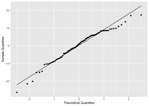

shapiro.test(model1_fitresid$.resid)


    Shapiro-Wilk normality test
data:  model1_fitresid$.resid
W = 0.97192, p-value = 0.07527

50 / 82

Model 2: prestige ~ education +  income1. Fit a model2. Visualise the fitted model3. Measure the strength of the fit4. Residual analysis51 / 82

Model 2: prestige ~ education + `income`

model2 <- lm(prestige ~ income + education, data=train)
summary(model2)


Call:
lm(formula = prestige ~ income + education, data = train)
Residuals:
     Min       1Q   Median       3Q      Max 
-18.9407  -4.1745   0.2026   4.9471  17.7176 
Coefficients:
              Estimate Std. Error t value Pr(>|t|)    
(Intercept) -7.5400414  3.4980062  -2.156   0.0342 *  
income       0.0015286  0.0003249   4.705  1.1e-05 ***
education    4.1452613  0.3937971  10.526  < 2e-16 ***
---
Signif. codes:  0 '***' 0.001 '**' 0.01 '*' 0.05 '.' 0.1 ' ' 1
Residual standard error: 7.765 on 77 degrees of freedom
Multiple R-squared:  0.7986,    Adjusted R-squared:  0.7934 
F-statistic: 152.7 on 2 and 77 DF,  p-value: < 2.2e-16

52 / 82

Model 2: prestige ~ education + `income` (cont.)

model2_fitresid <- augment(model2)
model2_fitresid

# A tibble: 80 x 10
   .rownames prestige income education .fitted .resid .std.resid   .hat .sigma
   <chr>        <dbl>  <int>     <dbl>   <dbl>  <dbl>      <dbl>  <dbl>  <dbl>
 1 medical.…     67.5   5180     12.8     53.4  14.1       1.85  0.0350   7.64
 2 welders       41.8   6477      7.92    35.2   6.61      0.865 0.0317   7.78
 3 commerci…     40.2   8780     11.1     52.0 -11.8      -1.54  0.0186   7.70
 4 economis…     62.2   8049     14.4     64.6  -2.42     -0.318 0.0378   7.81
 5 farmers       44.1   3643      6.84    26.4  17.7       2.33  0.0374   7.54
 6 receptio…     38.7   2901     11.0     42.7  -3.96     -0.520 0.0405   7.80
 7 sales.su…     41.5   7482      9.84    44.7  -3.19     -0.414 0.0177   7.81
 8 mail.car…     36.1   5511      9.22    39.1  -3.00     -0.390 0.0163   7.81
 9 taxi.dri…     25.1   4224      7.93    31.8  -6.69     -0.873 0.0257   7.78
10 veterina…     66.7  14558     15.9     80.8 -14.1      -1.90  0.0853   7.63
# … with 70 more rows, and 1 more variable: .cooksd <dbl>

53 / 82

Plot of residuals vs fitted values

linearity and constant variance?

54 / 82

Normality of residuals

ggplot(model2_fitresid, 
       aes(x=.resid))+
  geom_histogram(colour="white")+ggtitle("Distribution of Residuals")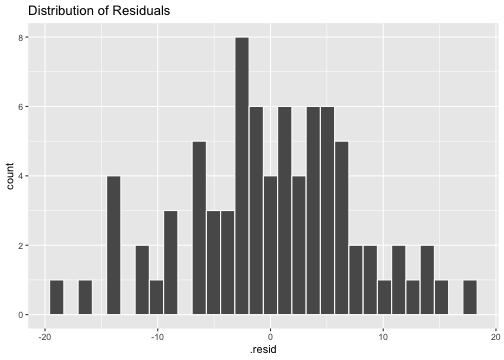

ggplot(model2_fitresid, 
       aes(sample=.resid))+
  stat_qq() + stat_qq_line()+labs(x="Theoretical Quantiles", y="Sample Quantiles")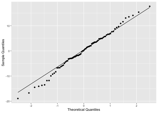

shapiro.test(model2_fitresid$.resid)


    Shapiro-Wilk normality test
data:  model2_fitresid$.resid
W = 0.99183, p-value = 0.8977

55 / 82

Plot of residuals vs predictor variables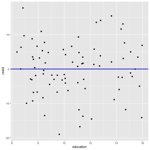

56 / 82

Model 3: prestige ~ education +  log(income)1. Fit a model2. Visualise the fitted model3. Measure the strength of the fit4. Residual analysis57 / 82

Model 3: prestige ~ education + `log(income)`

model3 <- lm(prestige ~ log(income) + education, data=train)
summary(model3)


Call:
lm(formula = prestige ~ log(income) + education, data = train)
Residuals:
     Min       1Q   Median       3Q      Max 
-17.5828  -4.1534   0.7978   4.3347  18.1881 
Coefficients:
            Estimate Std. Error t value Pr(>|t|)    
(Intercept) -86.5942    13.4064  -6.459 8.62e-09 ***
log(income)  10.2025     1.7189   5.936 7.91e-08 ***
education     4.2163     0.3436  12.271  < 2e-16 ***
---
Signif. codes:  0 '***' 0.001 '**' 0.01 '*' 0.05 '.' 0.1 ' ' 1
Residual standard error: 7.298 on 77 degrees of freedom
Multiple R-squared:  0.8221,    Adjusted R-squared:  0.8175 
F-statistic: 177.9 on 2 and 77 DF,  p-value: < 2.2e-16

model3_fitresid <- broom::augment(model3)

58 / 82

model3_fitresid <- broom::augment(model3)
model3_fitresid

# A tibble: 80 x 9
   .rownames prestige `log(income)` education .fitted .std.resid   .hat .sigma
   <chr>        <dbl>         <dbl>     <dbl>   <dbl>      <dbl>  <dbl>  <dbl>
 1 medical.…     67.5          8.55     12.8     54.6      1.79  0.0254   7.19
 2 welders       41.8          8.78      7.92    36.3      0.762 0.0341   7.32
 3 commerci…     40.2          9.08     11.1     53.0     -1.77  0.0202   7.20
 4 economis…     62.2          8.99     14.4     66.0     -0.536 0.0349   7.33
 5 farmers       44.1          8.20      6.84    25.9      2.54  0.0376   7.03
 6 receptio…     38.7          7.97     11.0     41.3     -0.364 0.0423   7.34
 7 sales.su…     41.5          8.92      9.84    45.9     -0.610 0.0203   7.33
 8 mail.car…     36.1          8.61      9.22    40.2     -0.562 0.0168   7.33
 9 taxi.dri…     25.1          8.35      7.93    32.0     -0.960 0.0255   7.30
10 veterina…     66.7          9.59     15.9     78.4     -1.66  0.0642   7.21
# … with 70 more rows, and 1 more variable: .cooksd <dbl>

If the variables used to fit the model are not included in data, then no .resid column will be included in the output.

When you transform variables (say a log transformation), augment will not display .resid column.

59 / 82

Add new variable (log.income) to the training set.

train$log.income. <- log(train$income)
model3 <- lm(prestige ~ log.income. + education, data=train)
model3_fitresid <- broom::augment(model3)
model3_fitresid

# A tibble: 80 x 10
   .rownames prestige log.income. education .fitted .resid .std.resid   .hat
   <chr>        <dbl>       <dbl>     <dbl>   <dbl>  <dbl>      <dbl>  <dbl>
 1 medical.…     67.5        8.55     12.8     54.6  12.9       1.79  0.0254
 2 welders       41.8        8.78      7.92    36.3   5.46      0.762 0.0341
 3 commerci…     40.2        9.08     11.1     53.0 -12.8      -1.77  0.0202
 4 economis…     62.2        8.99     14.4     66.0  -3.84     -0.536 0.0349
 5 farmers       44.1        8.20      6.84    25.9  18.2       2.54  0.0376
 6 receptio…     38.7        7.97     11.0     41.3  -2.60     -0.364 0.0423
 7 sales.su…     41.5        8.92      9.84    45.9  -4.40     -0.610 0.0203
 8 mail.car…     36.1        8.61      9.22    40.2  -4.07     -0.562 0.0168
 9 taxi.dri…     25.1        8.35      7.93    32.0  -6.92     -0.960 0.0255
10 veterina…     66.7        9.59     15.9     78.4 -11.7      -1.66  0.0642
# … with 70 more rows, and 2 more variables: .sigma <dbl>, .cooksd <dbl>

60 / 82

Plot of Residuals vs Fitted

Now - Model 3

Before - Model 2

61 / 82

Normality of residuals

ggplot(model3_fitresid, 
       aes(x=.resid))+
  geom_histogram(colour="white")+ggtitle("Distribution of Residuals")

ggplot(model3_fitresid, 
       aes(sample=.resid))+
  stat_qq() + stat_qq_line()+labs(x="Theoretical Quantiles", y="Sample Quantiles")

shapiro.test(model3_fitresid$.resid)


    Shapiro-Wilk normality test
data:  model3_fitresid$.resid
W = 0.9931, p-value = 0.9492

62 / 82

Plot of residuals vs predictor variables

63 / 82

Prestige vs income by type

R code: ___

Prestige vs income by type

R code: __

64 / 82

Model 4: prestige ~ education +  log(income) + type1. Fit a model2. Visualise the fitted model3. Measure the strength of the fit4. Residual analysis65 / 82

str(train)

'data.frame':    80 obs. of  7 variables:
 $ education  : num  12.79 7.92 11.13 14.44 6.84 ...
 $ income     : int  5180 6477 8780 8049 3643 2901 7482 5511 4224 14558 ...
 $ women      : num  76.04 5.17 3.16 57.31 3.6 ...
 $ prestige   : num  67.5 41.8 40.2 62.2 44.1 38.7 41.5 36.1 25.1 66.7 ...
 $ census     : int  3156 8335 5133 2311 7112 4171 5130 4172 9173 3115 ...
 $ type       : Factor w/ 3 levels "bc","prof","wc": 3 1 3 2 NA 3 3 3 1 2 ...
 $ log.income.: num  8.55 8.78 9.08 8.99 8.2 ...

66 / 82

Model 4: prestige ~ education + log(income) + `type`

model4 <- lm(prestige ~ log.income. + education + type, data=train)
summary(model4)


Call:
lm(formula = prestige ~ log.income. + education + type, data = train)
Residuals:
     Min       1Q   Median       3Q      Max 
-13.8420  -3.7790   0.6321   4.7393  17.8611 
Coefficients:
            Estimate Std. Error t value Pr(>|t|)    
(Intercept) -71.9102    17.7934  -4.041 0.000133 ***
log.income.   9.1505     2.2945   3.988 0.000160 ***
education     3.5136     0.7553   4.652 1.48e-05 ***
typeprof      6.7702     4.3797   1.546 0.126595    
typewc       -1.6497     3.0213  -0.546 0.586758    
---
Signif. codes:  0 '***' 0.001 '**' 0.01 '*' 0.05 '.' 0.1 ' ' 1
Residual standard error: 6.746 on 71 degrees of freedom
  (4 observations deleted due to missingness)
Multiple R-squared:  0.8494,    Adjusted R-squared:  0.8409 
F-statistic: 100.1 on 4 and 71 DF,  p-value: < 2.2e-16

67 / 82

Model 4: prestige ~ education + log(income) + `type`

model4_fitresid <- augment(model4)
head(model4_fitresid)

# A tibble: 6 x 11
  .rownames prestige log.income. education type  .fitted .resid .std.resid
  <chr>        <dbl>       <dbl>     <dbl> <fct>   <dbl>  <dbl>      <dbl>
1 medical.…     67.5        8.55     12.8  wc       49.6 17.9       2.78  
2 welders       41.8        8.78      7.92 bc       36.2  5.58      0.843 
3 commerci…     40.2        9.08     11.1  wc       48.6 -8.43     -1.32  
4 economis…     62.2        8.99     14.4  prof     67.9 -5.69     -0.862 
5 receptio…     38.7        7.97     11.0  wc       38.2  0.515     0.0802
6 sales.su…     41.5        8.92      9.84 wc       42.6 -1.14     -0.180 
# … with 3 more variables: .hat <dbl>, .sigma <dbl>, .cooksd <dbl>

68 / 82

Plot of Residuals vs Fitted

69 / 82

Normality of residuals

ggplot(model4_fitresid, 
       aes(x=.resid))+
  geom_histogram(colour="white")+ggtitle("Distribution of Residuals")

ggplot(model4_fitresid, 
       aes(sample=.resid))+
  stat_qq() + stat_qq_line()+labs(x="Theoretical Quantiles", y="Sample Quantiles")

shapiro.test(model4_fitresid$.resid)


    Shapiro-Wilk normality test
data:  model4_fitresid$.resid
W = 0.9838, p-value = 0.4445

70 / 82

Plot of residuals vs predictor variables

71 / 82

Multicollinearity

car::vif(model4)

                GVIF Df GVIF^(1/(2*Df))
log.income. 1.789890  1        1.337868
education   7.471481  1        2.733401
type        7.021948  2        1.627850

VIFs larger than 10 imply series problems with multicollinearity.

72 / 82

Detecting influential observations

library(lindia)
gg_cooksd(model4)

73 / 82

Influential outliers (cont.)

model4_fitresid %>%
  top_n(4, wt = .cooksd)

# A tibble: 4 x 11
  .rownames prestige log.income. education type  .fitted .resid .std.resid
  <chr>        <dbl>       <dbl>     <dbl> <fct>   <dbl>  <dbl>      <dbl>
1 medical.…     67.5        8.55      12.8 wc       49.6  17.9        2.78
2 veterina…     66.7        9.59      15.9 prof     78.6 -11.9       -1.84
3 file.cle…     32.7        8.01      12.1 wc       42.2  -9.53      -1.50
4 collecto…     29.4        8.46      11.2 wc       43.2 -13.8       -2.12
# … with 3 more variables: .hat <dbl>, .sigma <dbl>, .cooksd <dbl>

Solutions

Remove influential observations, and re-fit model.
Transform explanatory variables to reduce influence.
Use weighted regression to down weight influence of extreme observations.

74 / 82

Hypothesis testing

$Y = β_{0} + β_{1} x_{1} + β_{2} x_{2} + β_{3} x_{3} + β_{4} x_{4} + ϵ$

What is the overall adequacy of the model?

$H 0 : β_{1} = β_{2} = β_{3} = β_{4}$

$H 1 : β_{j} \neq 0 for at least one j, j = 1, 2, 3, 4$

Which specific regressors seem important?

$H 0 : β_{1} = 0$

$H 1 : β_{1} \neq 0$

75 / 82

Making predictions

Method 1

head(test)

                       education income women prestige census type
gov.administrators         13.11  12351 11.16     68.8   1113 prof
general.managers           12.26  25879  4.02     69.1   1130 prof
mining.engineers           14.64  11023  0.94     68.8   2153 prof
surveyors                  12.39   5902  1.91     62.0   2161 prof
vocational.counsellors     15.22   9593 34.89     58.3   2391 prof
physicians                 15.96  25308 10.56     87.2   3111 prof

test$log.income. <- log(test$income)

predict(model4, test)

##        gov.administrators          general.managers          mining.engineers 
##                  67.13432                  70.91638                  71.46917 
##                 surveyors    vocational.counsellors                physicians 
##                  57.84739                  72.23557                  83.71240 
##             nursing.aides               secretaries               bookkeepers 
##                  35.92664                  43.13913                  42.87183 
##           shipping.clerks       telephone.operators             office.clerks 
##                  36.14801                  37.10841                  41.15412 
##              sales.clerks service.station.attendant      real.estate.salesmen 
##                  33.68323                  34.08491                  46.41067 
##                 policemen                launderers              farm.workers 
##                  49.69682                  27.10663                  26.13155 
##         textile.labourers                machinists        electronic.workers 
##                  26.40488                  39.63996                  34.62981 
##                    masons 
##                  30.82164

76 / 82

Making predictions

Method 2

library(modelr)
test <- test %>% add_predictions(model4)
test

                          education income women prestige census type
gov.administrators            13.11  12351 11.16     68.8   1113 prof
general.managers              12.26  25879  4.02     69.1   1130 prof
mining.engineers              14.64  11023  0.94     68.8   2153 prof
surveyors                     12.39   5902  1.91     62.0   2161 prof
vocational.counsellors        15.22   9593 34.89     58.3   2391 prof
physicians                    15.96  25308 10.56     87.2   3111 prof
nursing.aides                  9.45   3485 76.14     34.9   3135   bc
secretaries                   11.59   4036 97.51     46.0   4111   wc
bookkeepers                   11.32   4348 68.24     49.4   4131   wc
shipping.clerks                9.17   4761 11.37     30.9   4153   wc
telephone.operators           10.51   3161 96.14     38.1   4175   wc
office.clerks                 11.00   4075 63.23     35.6   4197   wc
sales.clerks                  10.05   2594 67.82     26.5   5137   wc
service.station.attendant      9.93   2370  3.69     23.3   5145   bc
real.estate.salesmen          11.09   6992 24.44     47.1   5172   wc
policemen                     10.93   8891  1.65     51.6   6112   bc
launderers                     7.33   3000 69.31     20.8   6162   bc
farm.workers                   8.60   1656 27.75     21.5   7182   bc
textile.labourers              6.74   3485 39.48     28.8   8278   bc
machinists                     8.81   6686  4.28     44.2   8313   bc
electronic.workers             8.76   3942 74.54     50.8   8534   bc
masons                         6.60   5959  0.52     36.2   8782   bc
                          log.income.     pred
gov.administrators           9.421492 67.13432
general.managers            10.161187 70.91638
mining.engineers             9.307739 71.46917
surveyors                    8.683047 57.84739
vocational.counsellors       9.168789 72.23557
physicians                  10.138876 83.71240
nursing.aides                8.156223 35.92664
secretaries                  8.303009 43.13913
bookkeepers                  8.377471 42.87183
shipping.clerks              8.468213 36.14801
telephone.operators          8.058644 37.10841
office.clerks                8.312626 41.15412
sales.clerks                 7.860956 33.68323
service.station.attendant    7.770645 34.08491
real.estate.salesmen         8.852522 46.41067
policemen                    9.092795 49.69682
launderers                   8.006368 27.10663
farm.workers                 7.412160 26.13155
textile.labourers            8.156223 26.40488
machinists                   8.807771 39.63996
electronic.workers           8.279443 34.62981
masons                       8.692658 30.82164

add log.income to test

library(modelr)
test <- test %>% add_predictions(model4)

77 / 82

In-sample accuracy and out of sample accuracy

# test MSE
test %>%
add_predictions(model4) %>%
summarise(MSE = mean((prestige - pred)^2, na.rm=TRUE))

       MSE
1 40.82736

# training MSE
train %>%
add_predictions(model4) %>%
summarise(MSE = mean((prestige - pred)^2, na.rm=TRUE))

       MSE
1 42.51919

78 / 82

Out of sample accuracy: model 1, model 2 and model 3

# test MSE
test %>%
add_predictions(model1) %>%
summarise(MSE = mean((prestige - pred)^2, na.rm=TRUE))

       MSE
1 105.7605

# test MSE
test %>%
add_predictions(model2) %>%
summarise(MSE = mean((prestige - pred)^2, na.rm=TRUE))

       MSE
1 67.16647

# test MSE
test %>%
add_predictions(model3) %>%
summarise(MSE = mean((prestige - pred)^2, na.rm=TRUE))

       MSE
1 45.36052

Model 4: 42.51

79 / 82

Modelling cycle

EDA
Fit
Examine the residuals (multicollinearity/ Influential cases)
Transform/ Add/ Drop regressors if necessary
Repeat above until you find a good model(s)
Use out-of-sample accuracy to select the final model

Presenting results

EDA
Final regression fit:
- sample size
- estimated coefficients and standard errors
- $R_{a d j}^{2}$
- Visualizations (model fit, coefficients and CIs)
Model adequacy checking results: Residual plots and interpretations
Hypothesis testing and interpretations
- ANOVA, etc.
Out-of sample accuracy

Some flexibility is possible in the presentation of results and you may want to adjust the rules above to emphasize the point you are trying to make.

80 / 82

Other models

Decision trees
Random forests
XGBoost
Deep learning approaches and many more..

81 / 82

Slides available at: https://thiyanga.netlify.app/courses/rmsc2020/contentr/

82 / 82

Help

Keyboard shortcuts

↑, ←, Pg Up, k

Go to previous slide

↓, →, Pg Dn, Space, j

Go to next slide

Home

Go to first slide

End

Go to last slide

Number + Return

Go to specific slide

b / m / f

Toggle blackout / mirrored / fullscreen mode

Clone slideshow

Toggle presenter mode

Start & Stop the presentation timer

Reset the presentation timer

?, h

Toggle this help

STA 517 3.0 Programming and Statistical Computing with R

Regression Analysis

Dr Thiyanga Talagala

25 October 2020

Packages

Data: Prestige of Canadian Occupations

Data description

Training test and Test set

Exploratory Data Analysis

Exploratory Data Analysis

Exploratory Data Analysis

Exploratory Data Analysis

Exploratory Data Analysis

Exploratory Data Analysis

Exploratory Data Analysis

Exploratory Data Analysis

Exploratory Data Analysis

Exploratory Data Analysis

Exploratory Data Analysis

Regression analysis

Steps

Model 1: prestige ~ education

Recap

How to estimate β0β0 and β1β1?

Model 1: prestige ~ education

1. Fit a model

Model 1: Fit a model

What's messy about the output?

broom functions

Component-level statistics: tidy()

Component-level statistics: tidy() (cont.)

Why are tidy model outputs useful?

Model 1: prestige ~ education

1. Fit a model

2. Visualise the fitted model

Model 1: Visualise the fitted model

Model 1: Visualise the fitted model (style the line)

Model 1: prestige ~ education

1. Fit a model

2. Visualise the fitted model

3. Measure the strength of the fit

Model-level statistics: glance()

Model 1: prestige ~ education

1. Fit a model

2. Visualise the fitted model

3. Measure the strength of the fit

4. Residual analysis

Observation-level statistics: augment()

Residuals and Fitted Values

Residuals and Fitted Values

Conditions for inference for regression

Plot of residuals in time sequence.

Plot of residuals vs fitted values

Plot of residuals vs fitted values and Plot of residuals vs predictor

linearity and constant variance

Normality of residuals

Model 2: prestige ~ education + income

1. Fit a model

2. Visualise the fitted model

3. Measure the strength of the fit

4. Residual analysis

Model 2: prestige ~ education + income

Model 2: prestige ~ education + income (cont.)

Plot of residuals vs fitted values

Normality of residuals

Plot of residuals vs predictor variables

Model 3: prestige ~ education + log(income)

1. Fit a model

2. Visualise the fitted model

3. Measure the strength of the fit

4. Residual analysis

Model 3: prestige ~ education + log(income)

Plot of Residuals vs Fitted

Normality of residuals

Plot of residuals vs predictor variables

Prestige vs income by type

Prestige vs income by type

Model 4: prestige ~ education + log(income) + type

1. Fit a model

2. Visualise the fitted model

How to estimate $β_{0}$ and $β_{1}$ ?

`broom` functions

Component-level statistics: `tidy()`

Component-level statistics: `tidy()` (cont.)

Model-level statistics: `glance()`

Observation-level statistics: `augment()`

Model 2: prestige ~ education + `income`

Model 2: prestige ~ education + `income`

Model 2: prestige ~ education + `income` (cont.)

Model 3: prestige ~ education + `log(income)`

Model 3: prestige ~ education + `log(income)`

Model 4: prestige ~ education + log(income) + `type`

Model 4: prestige ~ education + log(income) + `type`

Model 4: prestige ~ education + log(income) + `type`