Logistic Regression: Model Building and Interpretation
Data
In this post I am going to use penguins dataset in palmerpenguins package in R. First we load the dataset.
library(palmerpenguins)
library(skimr)
library(tidyverse)
library(plotly)
library(visdat)
library(patchwork)
data("penguins")
Here is an overview of the dataset.
skim(penguins)| Name | penguins |
| Number of rows | 344 |
| Number of columns | 8 |
| _______________________ | |
| Column type frequency: | |
| factor | 3 |
| numeric | 5 |
| ________________________ | |
| Group variables | None |
Variable type: factor
| skim_variable | n_missing | complete_rate | ordered | n_unique | top_counts |
|---|---|---|---|---|---|
| species | 0 | 1.00 | FALSE | 3 | Ade: 152, Gen: 124, Chi: 68 |
| island | 0 | 1.00 | FALSE | 3 | Bis: 168, Dre: 124, Tor: 52 |
| sex | 11 | 0.97 | FALSE | 2 | mal: 168, fem: 165 |
Variable type: numeric
| skim_variable | n_missing | complete_rate | mean | sd | p0 | p25 | p50 | p75 | p100 | hist |
|---|---|---|---|---|---|---|---|---|---|---|
| bill_length_mm | 2 | 0.99 | 43.92 | 5.46 | 32.1 | 39.23 | 44.45 | 48.5 | 59.6 | ▃▇▇▆▁ |
| bill_depth_mm | 2 | 0.99 | 17.15 | 1.97 | 13.1 | 15.60 | 17.30 | 18.7 | 21.5 | ▅▅▇▇▂ |
| flipper_length_mm | 2 | 0.99 | 200.92 | 14.06 | 172.0 | 190.00 | 197.00 | 213.0 | 231.0 | ▂▇▃▅▂ |
| body_mass_g | 2 | 0.99 | 4201.75 | 801.95 | 2700.0 | 3550.00 | 4050.00 | 4750.0 | 6300.0 | ▃▇▆▃▂ |
| year | 0 | 1.00 | 2008.03 | 0.82 | 2007.0 | 2007.00 | 2008.00 | 2009.0 | 2009.0 | ▇▁▇▁▇ |
summary(penguins) species island bill_length_mm bill_depth_mm
Adelie :152 Biscoe :168 Min. :32.10 Min. :13.10
Chinstrap: 68 Dream :124 1st Qu.:39.23 1st Qu.:15.60
Gentoo :124 Torgersen: 52 Median :44.45 Median :17.30
Mean :43.92 Mean :17.15
3rd Qu.:48.50 3rd Qu.:18.70
Max. :59.60 Max. :21.50
NA's :2 NA's :2
flipper_length_mm body_mass_g sex year
Min. :172.0 Min. :2700 female:165 Min. :2007
1st Qu.:190.0 1st Qu.:3550 male :168 1st Qu.:2007
Median :197.0 Median :4050 NA's : 11 Median :2008
Mean :200.9 Mean :4202 Mean :2008
3rd Qu.:213.0 3rd Qu.:4750 3rd Qu.:2009
Max. :231.0 Max. :6300 Max. :2009
NA's :2 NA's :2 Before moving on to the full logistic regression model, it’s a good idea to look at the associations between each predictor and gender. Before moving on to the whole model, It’s critical to first grasp these linkages. We can use logistic regression to look at all of the predictors simultaneously.
p1_species <- penguins %>%
  na.omit() %>%
  count(species,sex) %>%
  group_by(species) %>%
  mutate(Percentage = 100*n/sum(n)) %>%
  ggplot(aes(x = species,y = Percentage,fill=sex))+
  geom_bar(stat="identity") +
  scale_fill_manual(values = c("purple","cyan4")) +
  coord_flip() +
  theme(legend.position = "bottom") +
  ggtitle("a")

p2_island <- penguins %>%
  count(island,sex) %>%
  group_by(island) %>%
  mutate(Percentage = 100*n/sum(n)) %>%
  ggplot(aes(x = island,y = Percentage,fill=sex))+
  geom_bar(stat="identity") +
  scale_fill_manual(values = c("purple","cyan4")) +
  coord_flip() +
  theme(legend.position = "bottom") +
  ggtitle("b")
(p1_species|p2_island)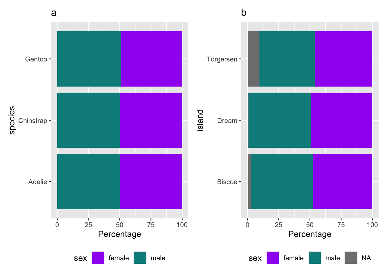
Figure 1: Distribution of (a) species and (d) island by gender.
p3_length <-  ggplot(penguins, aes(x=sex, y=bill_length_mm, fill=sex)) +
  geom_boxplot() +
  scale_fill_manual(values = c("purple","cyan4")) +
  theme(legend.position = "bottom") + ggtitle("a")

p4_depth <-  ggplot(penguins, aes(x=sex, y=bill_depth_mm, fill=sex)) +
  geom_boxplot() +
  scale_fill_manual(values = c("purple","cyan4")) +
  theme(legend.position = "bottom") + ggtitle("b")

p5_flipper <-  ggplot(penguins, aes(x=sex, y=flipper_length_mm, fill=sex)) +
  geom_boxplot() +
  scale_fill_manual(values = c("purple","cyan4")) +
  theme(legend.position = "bottom") + ggtitle("c")

p6_bmi <-  ggplot(penguins, aes(x=sex, y=body_mass_g, fill=sex)) +
  geom_boxplot() +
  scale_fill_manual(values = c("purple","cyan4")) +
  theme(legend.position = "bottom") + ggtitle("d")

(p3_length|p4_depth)/(p5_flipper|p6_bmi)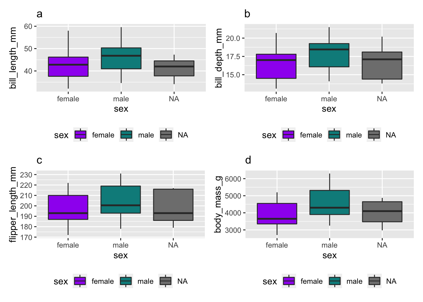
Figure 2: Distribution of (a) bill length, (b) bill depth, (c) flipper length and (d) body mass index by gender.
Missing values exploration
vis_miss(penguins)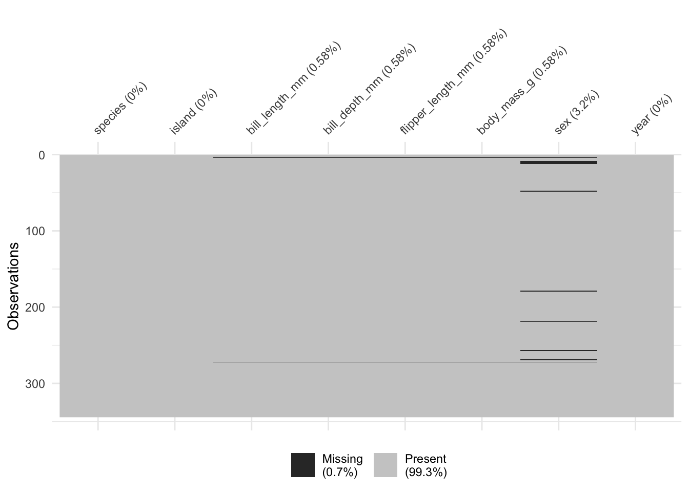
Remove missing values
penguins_omit <- penguins %>%
  na.omit()
vis_miss(penguins_omit)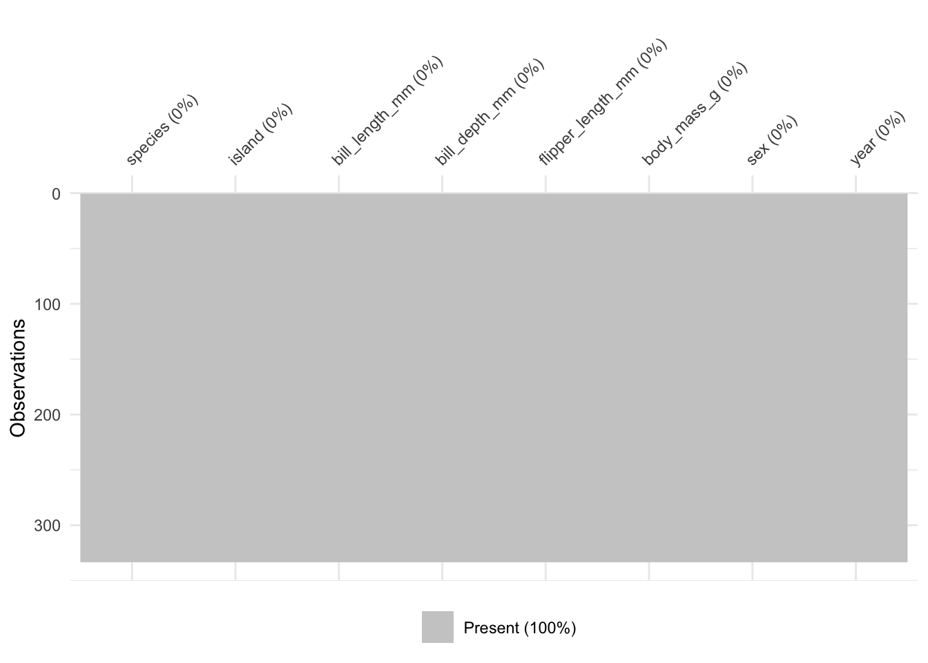
Building logistic regression
Then, using the other variables in the dataset, I’ll create a logistic regression model to predict the gender of the palmer penguins. One goal of this work is to identify which variables significantly contribute to determining the gender of penguins. Before beginning to build the model, double-check that all qualitative variables have been saved as factors.
fit <- glm(sex ~ species + island + bill_length_mm + bill_depth_mm + flipper_length_mm + body_mass_g, data=penguins_omit, family="binomial")
summary(fit)
Call:
glm(formula = sex ~ species + island + bill_length_mm + bill_depth_mm +
    flipper_length_mm + body_mass_g, family = "binomial", data = penguins_omit)

Deviance Residuals:
    Min       1Q   Median       3Q      Max
-3.4128  -0.2000   0.0022   0.1441   2.8235

Coefficients:
                    Estimate Std. Error z value Pr(>|z|)
(Intercept)       -80.376672  12.329735  -6.519 7.08e-11 ***
speciesChinstrap   -7.402697   1.662534  -4.453 8.48e-06 ***
speciesGentoo      -8.427611   2.597027  -3.245  0.00117 **
islandDream         0.324158   0.809135   0.401  0.68870
islandTorgersen    -0.507858   0.855746  -0.593  0.55287
bill_length_mm      0.614436   0.131968   4.656 3.22e-06 ***
bill_depth_mm       1.646446   0.335798   4.903 9.43e-07 ***
flipper_length_mm   0.026654   0.048307   0.552  0.58111
body_mass_g         0.005819   0.001087   5.352 8.71e-08 ***
---
Signif. codes:  0 '***' 0.001 '**' 0.01 '*' 0.05 '.' 0.1 ' ' 1

(Dispersion parameter for binomial family taken to be 1)

    Null deviance: 461.61  on 332  degrees of freedom
Residual deviance: 126.05  on 324  degrees of freedom
AIC: 144.05

Number of Fisher Scoring iterations: 7
To represent qualitative variables, R will build an indicator (dummy) variable using the lowest coded category as the reference group. For example,
\[Y=\begin{cases} 0, & \text{if female}\\ 1, & \text{if male} \end{cases}\]
Interpretation of parameter estimates of logistic regression
The “Estimates” in the above output corresponds to the log-odds. The odd ratios can be obtained as follows:
exp(coefficients(fit)) (Intercept) speciesChinstrap speciesGentoo islandDream
1.238383e-35 6.096066e-04 2.187435e-04 1.382866e+00
islandTorgersen bill_length_mm bill_depth_mm flipper_length_mm
6.017832e-01 1.848613e+00 5.188507e+00 1.027012e+00
body_mass_g
1.005836e+00 \[odd = \frac{P(event)}{1-P(event)}\]
The 95% confidence intervals for log-odds can be obtained as follows
confint.default(fit) 2.5 % 97.5 %
(Intercept) -1.045425e+02 -56.210836165
speciesChinstrap -1.066120e+01 -4.144190616
speciesGentoo -1.351769e+01 -3.337530854
islandDream -1.261718e+00 1.910034317
islandTorgersen -2.185089e+00 1.169372704
bill_length_mm 3.557834e-01 0.873088085
bill_depth_mm 9.882945e-01 2.304597483
flipper_length_mm -6.802606e-02 0.121333507
body_mass_g 3.687778e-03 0.007949886The 95% confidence intervals for odds are as follows
exp(confint.default(fit)) 2.5 % 97.5 %
(Intercept) 3.960644e-46 3.872077e-25
speciesChinstrap 2.343681e-05 1.585626e-02
speciesGentoo 1.346919e-06 3.552456e-02
islandDream 2.831672e-01 6.753321e+00
islandTorgersen 1.124677e-01 3.219972e+00
bill_length_mm 1.427298e+00 2.394293e+00
bill_depth_mm 2.686648e+00 1.002014e+01
flipper_length_mm 9.342361e-01 1.129001e+00
body_mass_g 1.003695e+00 1.007982e+00We can write the fitted logistic regression model as follows
\[\hat{Y} = \frac{1}{1+e^{-z}} = \frac{1}{e^{-80.83 -7.40Chinstrap -8.42Gentoo +0.32Dream -0.50Torgersen + 0.61 bill\_length\_mm + 1.64 bill\_depth\_mm + 0.02 flipper\_length\_mm + 0.005 body\_mass\_g}}\]
Where,
\[Chinstrap=\begin{cases} 1, & \text{if Chinstrap}\\ 0, & \text{otherwise} \end{cases}\]
\[Gentoo=\begin{cases} 1, & \text{if Gentoo}\\ 0, & \text{otherwise} \end{cases}\]
\[Dream=\begin{cases} 1, & \text{if Dream}\\ 0, & \text{otherwise} \end{cases}\]
\[Torgersen=\begin{cases} 1, & \text{if Torgersen}\\ 0, & \text{otherwise} \end{cases}\]
\[bill\_length\_mm = \text{bill length (millimeters)},\] \[bill\_depth\_mm = \text{bill depth (millimeters)},\]
\[flipper\_length\_mm = \text{flipper length (millimeters)},\]
\[body\_mass\_g = \text{body mass (grams)}.\]
Interpretation of parameter estimates
The variables species, bill length (mm), bill depth (mm) and body mass (g) significantly contribute to the model.
With all other factors held constant, this fitted model predicts that the odds of discovering a male penguin on Dream island are 1.38 times higher than on Biscoe island.
For each one-unit increase in bill depth, the odds of detecting a male increased 5.18 times (95 percent CI 2.68–10.02).
Model Evaluation: Next Post! Model evaluation should be done before interpreting the model.